Introduction to the Scipy Stack - Scientific Computing Tools
for Python
Marcel Oliver
Date: February 5, 2020
Abstract:
Over the last 15 years, an enormous and increasingly well integrated
collection of Python-based tools for Scientific Computing has
emerged--the
SciPy Stack or short
SciPy
[
7]. This document intends to provide a quick reference
guide and concise introduction to the core components of the stack.
It is aimed at beginning and intermediate
SciPy users and
does not attempt to be a comprehensive reference manual.
Python is a full-fledged general-purpose programming language with a
simple and clean syntax. It is equally well suited for expressing
procedural and object oriented programming concepts, has a powerful
standard library, numerous special purpose extension modules, and
interfaces well with external code. Python is interpreted (strictly
speaking, compiled to byte-code), ideal for interactive exploration.
As an interpreted language, Pythion cannot execute core numerical
algorithms at machine speed. This is where NumPy comes in:
since most large-scale computational problems can be formulated in
terms of vector and matrix operations, these basic building blocks are
provided with highly optimized compiled C or Fortran code and made
available from within Python as array objects. Thus, any
algorithm that can be formulated in terms of intrinsic operations on
arrays will run at near-native speed when operating on large data
sets. For those special cases where this is insufficient, Python
offers mechanisms for including compiled time-critical code sections,
ranging from in-lining a few lines of C to wrapping entire external
libraries into Python.
On top of NumPy, a collection of several large extension
libraries creates a very comprehensive, powerful environment for
Scientific Computing. SciPy extends the basic array
operations by providing higher-level tools which cover statistics,
optimization, special functions, ODE solvers, advanced linear algebra,
and more. Matplotlib is a plotting library which can create
beautiful and very flexible 2D graphics as well as basic 3D plots.
IPython is indispensable as an interactive shell and provides
a browser-based notebook interface. Further libraries include
pandas for data analysis, Mayavi for powerful 3D
visualization, and SymPy for symbolic mathematics; many more
specialized scientific libraries and applications are readily
available on the net.
At the same time, the whole universe of general-purpose Python
extensions is available to the SciPy developer. In
particular, xlrd and xlwr allow reading and writing
of Excel files and the csv module allows robust handling of
CSV data files. There are several comprehensive GUI toolkits,
libraries for network protocols, database access, and other tools
which help building complex stand-alone applications.
This document focuses on the use of NumPy, the SciPy
library, matplotlib, and IPython--together referred
to as the SciPy Stack or simply SciPy
[7]--for rapid prototyping of vectorizable numerical code.
In this capacity, SciPy competes with Matlab, a
proprietary development environment which has dominated Scientific
Computing for many years but it is increasingly challenged by
SciPy for a number of reasons:
- Python is an appealing programming language. It is conceptually
clean, powerful, and scales well from interactive experimentation all
the way to building large code bases. The Matlab language,
on the other hand, was optimized for the former at the expense of the
latter.
- SciPy is free software. You can run it on any machine,
at any time, for any purpose. And, in principle, the code is fully
transparent down to machine level, which is how science should be
done. Matlab, on the other hand, must be licensed. Licenses
typically come with number-of-CPU restrictions, site licenses require
network connection to the license server, and there are different
conditions for academic and for commercial use. Moreover, its
numerical core is not open to public scrutiny. (There is also
Octave, a free clone of Matlab. Unfortunately, it
is strictly inferior to Matlab while sharing its conceptual
disadvantages.)
- Numerical Python array objects work cleanly in any
dimension. Powerful slicing and “broadcasting” constructs make
multi-dimensional array operations very easy. Matlab, on the
other hand, is highly optimized for the common one- and
two-dimensional case, but the general case is less idiomatic.
- matplotlib produces beautiful production-quality
graphics. Labels can be transparently typeset in TEX, matching the
rest of the document. In addition, there is great flexibility, e.g.,
for non-standard coordinate axes, non-numerical graphical elements,
inlays, and customized appearance. Matlab graphics are
powerful and well-integrated into the core system, but rather less
flexible and aesthetically appealing.
So what are the drawbacks of SciPy? In practice, very few.
Documentation is scattered and less coherent than Matlab's.
When working offline, the help system is not always sufficient,
especially if you do not know the precise name of a function you are
looking for. This is compensated, to some extend, by lots of high
quality resources on the internet. And this document tries to address
some of the documentation gaps for newcomers to SciPy.
For the simplest use cases, working in Python exacts a small tribute
in the form of increased complexity (name space separation, call by
reference semantics). However, in relation to the associated increase
in expressive power, it is a very small price to pay and handled by
Python in a minimally intrusive way.
There are other considerations, both in favor of and against Python
which can easily be found on the net. They are are mostly tied to
specific domains of application--the above is what matters most for
general purpose Scientific Computing.
Unless you have legacy code, install the stack based on Python 3.
Python 2.7 is increasingly unmaintained and should not be used. On
Linux, install spyder which will pull in all the software you
need. (yum install python3-spyder on Redhat-based and
apt-get install python3-spyder on Debian-based
distributions.)
On Windows and MacOS, install the Anaconda Python
distribution [4] (also available for Linux, but using
distribution packages is often better).
2.2 IPython and Spyder
The Ipython shell provides a powerful command line interface
to the SciPy Stack. We always invoke it as
ipython3 --pylab
The command line option --pylab loads numpy and
matplotlib into the global name space. (In general, python
modules must be loaded explicitly.) It also modifies the threading
model so that the shell does not block on plotting commands.
When writing scripts, you will have to load the modules you use
explicitly. More on this in Section 3.1.
Spyder integrates a text editor, help browser, and
interactive Ipython shell in one application. Make sure that
the shell starts up with the --pylab option: Go to
Tools-Preferences-Ipython console-Graphics and check the boxes
“Activate support” and “Automatically load Pylab and NumPy
modules”. You may also want to set “Backend” to “Automatic” to
enable graphics in a separate window for zooming and panning.
- help(name) explains the variable or function
name.
- help() enters a text-based help browser, mainly useful
for help on the Python language core.
- help(pylab) displays help information on
Matlab-style plotting commands.
quickref displays a summary of Ipython shell
features.
- The default is one command per line without an explicit line
termination character, but you may use
- ; to separate several commands within a line,
\ to continue an expression into the next line; may be
omitted if the continuation is unambiguous.
- Comments are preceded by #.
- Python is case-sensitive.
- Code blocks are grouped by level of indentation! See
Section 5 on control structures below.
  In [1]: 'ab' \
     ...: 'cd'   # Explicit line continuation
  Out[1]: 'abcd'

  In [2]: min(1,
     ...:     0) # Implicit line continuation
  Out[2]: 0
2.5 Variables and simple expressions
- varname = expression assigns the result of
expression to varname.
- Some standard mathematical operators and functions: +,
-, *, /, **, sin,
cos, exp, arccos, abs, etc.
- Comparison operators are <, <=, >,
>=, ==, and !=.
- Boolean logical operators and, or,
not.
- The operators & and | represent
bit-wise AND and OR, respectively!
  In [1]: 10**2 - 1e2
  Out[1]: 0.0

  In [2]: sqrt(-1)
  Out[2]: nan

  In [3]: sqrt(-1+0j)
  Out[3]: 1j
Note: The last example shows that you have to force the use of complex
numbers. This behavior is different from Matlab.
All assignment in Python is by reference, not by value. When working
with immutable objects such as numerical constants, Python
automatically forces a copy, so the assignment-by-reference semantics
is somewhat hidden. However, when working with mutable objects
such as an array representing a vector or a matrix, one must
force a copy when required! This behavior is a source of
hard-to-discover bugs and will be discussed in detail in
Section 8.
Some commands useful for debugging:
Note: the commands above (except for del) are so-called
Ipython magic functions. Should you happen to overwrite them
with python function definitions, you still access them by prepending
%.
To record the execution time of single code snippets or whole
programs, several options are available. For most purposes, timing
from the Iphython shell suffices, but you can also put timing
instrumentation into any program code.
  In [1]: %timeit sum(arange(100))
  100000 loops, best of 3: 10.8 us per loop

  In [2]: %timeit sum(arange(10000))
  10000 loops, best of 3: 33.1 us per loop
  import time
  t = time.process_time()
  # Now do some big computation
  print "Elapsed CPU Time:", time.process_time() - t
Note: use time.monotonic() instead of
time.process_time() if you need wall-clock time.
If you need a thorough analysis of small time-critical sections of
code, use the timeit module:
  import timeit
  def f(x):
      # do something which needs to be timed
  t = timeit.Timer ('f(3.0)', 'from __main__ import f')
  print ("1000 Evaluations take", t.timeit(number=1000), "s")
Note: The timeit module runs f in a controlled environment,
so you have to set up the environment with the import statement. If
you need to pass variables as arguments, they need to be imported,
too.
Except for very simple exploratory code, the normal workflow involves
writing program code in separate text files and running them from the
Ipython shell. We only discuss the case where the code is so
simple as to be reasonably organized in a single file. You can easily
modularize larger projects; consult the Python language documentation
for details.
Program files should, but need not, carry the suffix .py. It
is common practice to start the first line with
#! /usr/bin/env python3
This allows direct execution of the file on Unix-like operating; on
other operating systems, it is simply ignored.
3.1 Module Import
When working with script files, you are responsible for module
loading. On the one hand, module import requires some explicit
attention (“where is my function?!”). On the other hand, module
namespaces provide sanity to complex projects and should be considered
one of the strong points of working with Python.
Since Python makes it is possible to import the same function or
module in different ways, it is important to standardize on some
convention. We suggest the following:
from pylab import *
This import statement sets up a large set of basic, often
Matlab-like functions in the current namespace. It is the
script file equivalent of starting the Ipython shell with the
pylab command line option as described in
Section 2.2.
If a more specialized function is required, we import it by its
explicit name into the current namespace. E.g., we write
from scipy.linalg import lu
to make available the function scipy.linalg.lu as
lu. This convention keeps the program code very close what
you would do in the interactive shell after invoking ipython
-pylab, and it also replicates Matlab to some extent.
All examples in this document use this convention!
When working on large projects, library modules, or programs where
only a small fraction of the code is numerical, we recommend using
full module path names, respectively their commonly used
abbreviations. E.g.,
  import numpy as np
  import matplotlib.pyplot as plt
  import scipy.linalg
Then the common functions arange, figure,
solve, all described further below, must be called as
np.arange, plt.figure, and
scipy.linalg.solve, respectively.
array objects representing vectors, matrices, and
higher-dimensional tensors are the most important building blocks for
writing efficient numerical code in Python. (numpy has an
alternative matrix data type more similar to the
Matlab matrix model. However, its use is discouraged
[6] and will not be discussed here.)
4.1 Vectors
  In [1]: linspace(0,1,5)
  Out[1]: array([ 0.  ,  0.25,  0.5 ,  0.75,  1.  ])

  In [2]: arange(0,1,0.25)
  Out[2]: array([ 0.  ,  0.25,  0.5 ,  0.75])

  In [3]: arange(5)
  Out[3]: array([0, 1, 2, 3, 4])

  In [4]: arange(1,6)
  Out[4]: array([1, 2, 3, 4, 5])

  In [5]: arange(1,6,dtype=float)
  Out[5]: array([ 1.,  2.,  3.,  4.,  5.])
Note that arange follows the general Python convention of
excluding the end point. The advantage of this convention is that the
vector arange(a,b) has  components when this difference
is integer.
components when this difference
is integer.
A matrix
 is generated as follows.
  In [1]: A = array([[1,2],[3,4]]); A
  Out[1]:
  array([[1, 2],
         [3, 4]])
Matrices can assembled from submatrices:
  In [2]: b = c_[5:7]; M = c_[A,b]; M
  Out[2]:
  array([[1, 2, 5],
         [3, 4, 6]])

  In [3]: M = r_[A,b[newaxis,:]]; M
  Out[3]:
  array([[1, 2],
         [3, 4],
         [5, 6]])
There are functions to create frequently used
 matrices.
If
matrices.
If  , only one argument is necessary.
- eye(m,n) produces a matrix with ones on the main
diagonal and zeros elsewhere. When , the identity matrix is
generated.
- rand(m,n) generates a random matrix whose entries are
uniformly distributed in the interval
 .
.
- zeros((m,n)) generates the zero matrix of dimension
.
- ones((m,n)) generates an matrix where all
entries are
 .
.
- diag(A) creates a vector containing the diagonal
elements
 of the matrix A.
- diag(v) generates a matrix with the elements from the
vector v on the diagonal.
- diag(v,k) generates a matrix with the elements from the
vector v on the k-th diagonal.
4.3 Basic matrix arithmetic
- The usual operators +, -, and *,
etc., act element-wise.
- A.T denotes the transpose of A.
- A.conj().T conjugates and transposes A.
- dot(A,B) computes the matrix product
 of two
matrices A and B.
of two
matrices A and B.
- A@v or dot(A,v) computes the product of a
matrix A with a vector v.
  In [1]: A = array([[1,2],[3,4]]); A-A.T
  Out[1]:
  array([[ 0, -1],
         [ 1,  0]])

  In [2]: A*A.T  # Element-wise product
  Out[2]:
  array([[ 1,  6],
         [ 6, 16]])

  In [3]: A@A.T  # Matrix product
  Out[3]:
  array([[ 5, 11],
         [11, 25]])
If the column vectors
 are represented by
one-dimensional arrays v and w, then
are represented by
one-dimensional arrays v and w, then
- v@w or dot(v,w) computes the inner product
 ;
;
c_[v]@r_[[w]] or outer(v,w) computes the outer
product  .
.
- sum(A) computes the sum of all elements of A.
- sum(A,axis=i) computes the sum along axis i of
the array.
- cumsum, prod, and cumprod follow the
same pattern for cumulative sums (an array with all
stages of intermediate summation), products, and cumulative products.
- trace(A) or A.trace() yields the trace of a
matrix A.
Note that the first axis (row indices for matrices) corresponds to
axis=0, the second (column indices for matrices) corresponds
to axis=1, etc.
  In [1]: A = array([[1,2],[3,4]]); sum(A)
  Out[1]: 10

  In [2]: sum(A,axis=0)
  Out[2]: array([4, 6])

  In [3]: sum(A,axis=1)
  Out[3]: array([3, 7])

  In [4]: cumprod(A)
  Out[4]: array([ 1,  2,  6, 24])
You can compute with Booleans where
False and
True
and
True . So the following expression
counts the number of nonzero elements of a matrix:
. So the following expression
counts the number of nonzero elements of a matrix:
  In [4]: A = eye(3); sum(A!=0)
  Out[4]: 3
- amax(A) or A.max() finds the maximum value in
the array A. You can add an axis argument as for
sum.
- argmax(A) or A.argmax() returns the index
relative to the flattened array A of only the
first element which takes the maximum value over the array. Works
also along a specified axis.
- fmax(A,B) element-wise max functions for two
arrays A and B.
- There is a corresponding set of min-functions.
- allclose(A,B) yields true if all elements of
A and B agree up to a small tolerance.
- around(A,decimals=n) or A.round(n) rounds the
elements of A to n decimal places.
  In [1]: A = array([[1,2],[3,4]]); amax(A); argmax(A)
  Out[1]: 4
  Out[1]: 3

  In [2]: A.flatten()[argmax(A)]
  Out[2]: 4

  In [3]: B = 3*eye(2); argmin(B,axis=1)
  Out[3]: array([1, 0])

  In [4]: fmax(A,B)
  Out[4]:
  array([[ 3.,  2.],
         [ 3.,  4.]])
Python indexing starts from zero! This is often different from
traditional mathematical notation, but has advantages [1].
  In [1]: A = array([[1,2],[3,4]]); A[0,0]
  Out[1]: 1

  In [2]: A[1]
  Out[2]: array([3, 4])

  In [3]: A[:,1]
  Out[3]: array([2, 4])
- a:b specifies the index range
 . Negative
values count from the end of the array.
. Negative
values count from the end of the array.
- a:b:s is the same in steps of s. When
s is negative, the order is reversed.
- delete(A,i,axis) deletes the subarray of index
i with respect to axis axis.
  In [1]: a = arange(5); a[2:]; a[-3:]; a[::-1]
  Out[1]: array([2, 3, 4])
  Out[1]: array([2, 3, 4])
  Out[1]: array([4, 3, 2, 1, 0])

  In [2]: A = eye(4, dtype=int); A[1:3,:3] = -8; A
  Out[2]:
  array([[ 1,  0,  0,  0],
         [-8, -8, -8,  0],
         [-8, -8, -8,  0],
         [ 0,  0,  0,  1]])

  In [3]: A[1:3,1:3] = eye(2, dtype=int)[::-1]; A
  Out[3]:
  array([[ 1,  0,  0,  0],
         [-8,  0,  1,  0],
         [-8,  1,  0,  0],
         [ 0,  0,  0,  1]])
- A.shape returns a python tuple containing the number of
elements in each dimension of the array A.
- A.size returns the total number of elements of
A.
- len(A) returns the number of elements of the
leftmost index of A.
  In [1]: A=eye(3); A.shape
  Out[1]: (3, 3)

  In [2]: A.size
  Out[2]: 9

  In [3]: len(A)
  Out[3]: 3
- A.reshape(i,j,...) transforms A into an array
of size (i,j,...). The total size must remain unchanged.
- A.flatten() flattens A into a 1-dimensional
array.
  In [1]: A = arange(12); B = A.reshape(2,3,2); B
  Out[1]:
  array([[[ 0,  1],
          [ 2,  3],
          [ 4,  5]],

         [[ 6,  7],
          [ 8,  9],
          [10, 11]]])

  In [2]: B.flatten()
  Out[2]: array([ 0,  1,  2,  3,  4,  5,  6,  7,  8,  9, 10, 11])
A powerful way to write short, elegant code is to use arrays of
integers or Booleans to index other arrays. Though our examples only
scratch the surface, many tricky index problems can be solved this
way!
- v[i], where i is a one-dimensional integer
array, yields an array of length len(i) containing elements
 .
.
- More generally, A[i,j,...] gives an array of shape
i.shape which must coincide with j.shape, etc., with
elements picked from A according to the indices at each
position of i, j, etc.
- A[b], where b is a Boolean array of the same
shape as A selects those components of A, for which
b is true.
Select every second element from an array a:
  In [1]: a = 2**arange(8); a
  Out[1]: array([  1,   2,   4,   8,  16,  32,  64, 128])

  In [2]: i = 2*arange(4); i
  Out[2]: array([0, 2, 4, 6])

  In [3]: a[i]
  Out[3]: array([ 1,  4, 16, 64])
Note: this particular example is equivalent to a[::2], but
the index array construct is much more general.
In two dimensions, index arrays work as follows. As an example, we
extract the main anti-diagonal of the matrix A:
  In [4]: A = arange(16).reshape(4,4); A
  Out[4]:
  array([[ 0,  1,  2,  3],
         [ 4,  5,  6,  7],
         [ 8,  9, 10, 11],
         [12, 13, 14, 15]])

  In [5]: i=arange(4); j=i[::-1]; A[i,j]
  Out[5]: array([ 3,  6,  9, 12])
Set all zero elements of A to  :
:
  In [6]: A = eye(3, dtype=int); A[A==0] = 2; A
  Out[6]:
  array([[1, 2, 2],
         [2, 1, 2],
         [2, 2, 1]])
When performing element-wise operations on a pair of arrays with a
different number of axes, Numpy will try to “broadcast” the smaller
array over the additional axis or axes of the larger array provided
this can be done in a compatible way. (Otherwise, an error message is
raised.)
  In [1]: A=ones((3,3)); b=arange(3); A*b
  Out[1]:
  array([[ 0.,  1.,  2.],
         [ 0.,  1.,  2.],
         [ 0.,  1.,  2.]])
The detailed general rules can be found in the Numpy documentation
[5]. However, you can also explicitly control how
broadcasting is done by inserting the keyword newaxis into
the index range specifier to indicate the axis over which this array
shall be broadcast. The above example is equivalent to the
following.
  In [2]: A*b[newaxis,:]
  Out[2]:
  array([[ 0.,  1.,  2.],
         [ 0.,  1.,  2.],
         [ 0.,  1.,  2.]])
In the same way, we can have b be broadcast over columns
rather than rows:
  In [3]: A*b[:,newaxis]
  Out[3]:
  array([[ 0.,  0.,  0.],
         [ 1.,  1.,  1.],
         [ 2.,  2.,  2.]])
Finally, a more complicated example using explicit broadcasting
illustrates how to compute general outer products for tensors of any
shape:
  In [4]: A=array([[1,2],[3,5]]); b=array([7,11]); \
     ...: A[:,newaxis,:]*b[newaxis,:,newaxis]
  Out[4]:
  array([[[ 7, 14],
          [11, 22]],

         [[21, 35],
          [33, 55]]])
- mean(a), var(a), and std(a) compute
mean, variance, and standard deviation of all array elements of the
array a. To compute them only along a specified axis, add an
axis-argument as described in
Section 4.3.
- random(shape) produces an array of random numbers drawn
from a uniform distribution on the interval
 with specified
shape.
with specified
shape.
- normal(m,s,shape) produces an array of random numbers
drawn from a normal distribution with mean m and standard
deviation s with specified shape.
- Similarly, you can draw from a binomial,
poisson, or exponential distribution. Consult the
help system for information on parameters.
The following numerical linear algebra functions are loaded into the
global namespace when you import pylab.
solve(A,b) yields the solution to the linear system  .
.
- inv(A) computes the inverse of
 .
.
- d,V = eig(A) computes a vector
 containing the
eigenvalues of and a matrix
containing the
eigenvalues of and a matrix  containing the corresponding
eigenvectors such that
containing the corresponding
eigenvectors such that  where
where
 .
.
- U,s,Vh = svd(A) computes the singular value
decomposition of . Returned are the matrix of left singular
vectors
 , the vector of corresponding singular values, and the
Hermitian complement of the right singular vectors
, the vector of corresponding singular values, and the
Hermitian complement of the right singular vectors
 . Then
  where
where
 .
.
- Q,R = qr(A) computes the QR-decomposition
 .
.
- norm(A) computes the Frobenius norm of an array of
any dimension; if is a matrix, norm(A,p) computes the
operator
 -norm, can only take the values 1, 2
or inf; if
-norm, can only take the values 1, 2
or inf; if  is a one-dimensional array, norm(v,p)
computes the vector -norm.
is a one-dimensional array, norm(v,p)
computes the vector -norm.
- cond(A) computes the condition number of with
respect to the -norm.
  In [1]: A = array([[0,1],[-2,0]]); eig(A)
  Out[1]:
  (array([ 0.+1.41421356j,  0.-1.41421356j]),
   array([[ 0.00000000-0.57735027j,  0.00000000+0.57735027j],
         [ 0.81649658+0.j        ,  0.81649658+0.j        ]]))

  In [2]: d,V = eig(A); allclose(dot(A,V), dot(V,diag(d)))
  Out[2]: True

  In [3]: svd(A)
  Out[3]:
  (array([[ 0.,  1.],
         [ 1.,  0.]]),
   array([ 2.,  1.]),
   array([[-1., -0.],
         [ 0.,  1.]]))

  In [4]: U,s,Vh = svd(A); allclose(dot(dot(U,diag(s)),Vh),A)
  Out[4]: True
The scipy.linalg module contains many more specialized
numerical linear algebra routines such as LU and Cholesky
factorization, solvers for linear systems with band-matrix structure,
matrix exponentials, the conjugate gradient method, and many more. To
get an overview, type
  In [1]: from scipy import linalg

  In [2]: help linalg
Contrary to Matlab behavior, solve(A,b) exits with
an error message when the matrix A is singular. If you need
a least-square or least-norm solution, you have to use lstsq
from scipy.linalg. This is illustrated in the following:
  In [1]: A = array([[1,0],[0,0]]); b=array([1,0]); c=b[::-1]

  In [2]: x = solve(A,b)
  LinAlgError: Singular matrix

  In [3]: from scipy.linalg import lstsq

  In [4]: x, res, rk, s = lstsq(A,b); x
  Out[4]: array([ 1.,  0.])
This example is an underdetermined system; any vector
 would solve the system. lstsq returns the least-norm
solution as well as the residual res, the effective rank of
the matrix rk, and the vector of singular values s.
When the system is inconsistent, the least-square solution is
returned:
would solve the system. lstsq returns the least-norm
solution as well as the residual res, the effective rank of
the matrix rk, and the vector of singular values s.
When the system is inconsistent, the least-square solution is
returned:
  In [5]: x, res, rk, s = lstsq(A,c); x
  Out[5]: array([ 0.,  0.])
5 Control structures
Conditional branching works as follows:
  if i<2:
      print("i is less than 2")
  elif i>=4:
      print("i is greater or equal to 4")
  else:
      print("i is greater or equal to 2 and less than 4")
A simple “for-loop” in Python works as follows, with the usual
conventions for the range specifier.
  In [1]: for i in range(3,5):
   ...:     print(i)
  3
  4
More generally, Python loops can iterate over many list-like objects
such as arrays:
  In [1]: a = exp(0.5j*pi*arange(4))

  In [2]: for x in a:
     ...:     print(x)

  (1+0j)
  (6.12303176911e-17+1j)
  (-1+1.22460635382e-16j)
  (-1.83690953073e-16-1j)
Here is an example of a while-loop:
  x = 5
  while x > 0:
     print(x)
     x -= 1
- Use break to leave the innermost loop (or, more
generally, the innermost scope);
- Use continue to go to the next iteration of the loop
without evaluating the remainder of its body;
- A loop can have an else:-clause which is run after a
loop terminates regularly, but will not be run if the loop is left via
a break-statement.
5.3 Functions
Functions are defined with the keyword def.
  In [1]: def square(x):
     ...:     return x*x

  In [2]: square(5)
  Out[2]: 25
Note: If a function does not take any arguments, its definition must
still end with parentheses. Functions do not need to return anything;
the return keyword is optional. Variables used within a
function are local--changing them locally does not change a
possibly globally defined variable of the same name.
If you pass a reference to a mutable object as a function argument,
you can still modify its data from within the function even though you
cannot modify the reference pointer itself. However, immutable
objects cannot be modified this way! This subtle difference is
explained more fully in Section 8.
Many standard mathematical functions such as sin or
abs are so-called universal functions which operate on arrays
element-wise. A newly defined function f (unless it consists
of nothing more than an arithmetic expression consisting only of
universal functions) will not do this, but it can be “vectorized”
via
f = vectorize(f)
so that it starts acting on arrays element-wise. Note that this
construct is for convenience, not for performance.
Arguments can be given a default value. The values of such optional
arguments can be specified either via an ordered argument list or as
an explicitly named keyword argument:
  In [1]: def root(x,q=2.0):
     ...:     return x**(1.0/q)

  In [2]: root(2), root(2,3), root(2,q=3)
  Out[2]: (1.4142135623730951, 1.2599210498948732, 1.2599210498948732)
Use global name to declare name as a global
variable.
  In [1]: def f():
     ...:     global a
     ...:     a = pi

  In [2]: a=1; f(); a
  Out[2]: 3.141592653589793
In Python, it is possible to nest function definitions. Further,
references to functions can be passed as references--this works just
like the reference passing for data objects.
The following example is called a closure where the function
defined in the inner scope has access to a local variable from the
enclosing scope, but the inner function is executed only after the
execution of the enclosing scope has finished.
  In [1]: def outer(xo):
     ...:     def inner(xi):
     ...:         return xo+xi
     ...:     return inner

  In [2]: f = outer(5)

  In [3]: f(3)
  Out[3]: 8
- plot(y) plots the values of the vector y with
the array index as
 -coordinates.
- plot(x,y) plots a polygonal line between points whose
-coordinates are supplied in the vector x and whose
 -coordinates are supplied in the vector y.
- plot(x,y,'g:') does the same with a green dotted line.
For a full list of format strings, consult help(plot).
- semilogx plots with logarithmic scaling on the
-axis, semilogy has logarithmic scaling on the -axis,
and loglog on both axes.
- xlim(xmin,xmax) sets limits xmin and
xmax for the -axis; use ylim to set limits for the
-axis.
- xlabel('x') and ylabel('y') set the labels on
the and -axis, respectively;
- title('title') sets a title for the whole plot;
- legend(('first graph','second graph'),loc='lower
right') inserts a legend in the lower right corner of the plot with
given labels for the first two graphs. For full information on
location strings and other options, consult help(legend);
- annotate('string',(x,y)) places an annotation string at
coordinate location (x,y).
It is possible to use TEX-style mathematical notation: enclose
mathematical expressions with $-signs. Important: since
TEX-commands and special characters are prefixed by a backslash,
which is usually interpreted by Python as a string escape, use “raw
strings” for all TEX-containing strings, e.g.,
title(r'$f(\theta) = \sin(\theta)$')
- figure() starts a new plot. (Ipython will open the
first figure for you, but subsequent plots will go into the same
coordinate axis, so when writing scripts, it is good practice to
always start out with the figure()-command.)
- show() displays all figures generated so far. (Ipython
will do this automatically for you, but script files will work
independently only if you close your plotting code with an explicit
show()-command.)
- subplot(325) creates a division of the figure into
 rows and columns of subplots, and sets up the the
  th plot
(counting from the top left) for current plotting.
th plot
(counting from the top left) for current plotting.
- savefig('filename.pdf') saves your current figure
in PDF format.
The Matplotlib plotting package includes simple 3D graphics (for more
sophisticated 3D modeling, Mayavi goes much beyond what Matplotlib can
do) which has to be imported explicitly via
from mpl_toolkits.mplot3d import Axes3D
To start a 3D plot, or more generally, a subplot, write
ax = subplot(111, projection='3d')
Then use
ax.plot_surface for a surface plot,
- ax.plot for a parametric curve,
- ax.scatter for a scatter plot.
Consult the documentation for arguments; a simple function plotting
example is given in Section 9.2 below.
- print('string') or print(a, b, c) to print a
line of console output. A new line is started automatically, and
print inserts one space between comma-separated arguments.
- input('Prompt:') accepts a string of data from the
console (ended with a newline) and returns the string.
Python has a powerful format string syntax. A format string is of the
form {name:format} where name is either a named
argument or argument position number and format is the format
specifier. Useful format specifiers are
3d
| Integer of characters width |
| +4d |
Integer width  , print sign whether
number is positive or negative , print sign whether
number is positive or negative |
| .6e |
Scientific notation,  decimal places decimal places |
| 8.3f |
Fixed point number of total width  and
decimal places and
decimal places |
| 8.3g |
Choose best format for total width and significant
digits |
  In [1]: '|{0:+4d}|{1:4d}|{n:8d}|'.format(22,33,n=-44)
  Out[1]: '| +22|  33|     -44|'

  In [2]: '|{pi:10.3e}|{e:10.3f}|{r:10.3g}|'.format(r=sqrt(2),**locals())
  Out[2]: '| 3.142e+00|     2.718|      1.41|'
To open a plain text file for reading, issue
f = open('test.txt', 'r')
To read the file contents, one often iterates over its lines as
follows:
  for line in f:
      print(line)
Files are automatically closed when the file object goes out of scope,
or can be explicitly closed by issuing f.close().
To open a plain text file for writing, issue
f = open('test.txt', 'w')
This will overwrite an already existing file! If you need to
append to a file, use 'a' as the mode string.
f.write('This is line ' + str(1) + '\n')
writes the line This is line 1. Note that you have to insert
explicit line termination characters '\n' to terminate a line.
write accepts only strings, so you have explicitly convert
other objects to strings using str. Note further that Python
has an internal I/O buffer, so if you want a guaranteed update of the
data on the file system, you must issue
f.flush()
This is often useful when writing log files during long-running
computations which are to be monitored via Unix tail or
similar utilities. Explicitly closing the file also flushes the I/O
buffer.
- savetxt('mydata.txt', a) saves the one or
two-dimensional array a into the file named
mydata.txt.
- a=loadtxt('mydata.txt') loads the file
mydata.txt containing plain text array data.
When you wish to save array data which only needs to be readable by
other SciPy instances, it is often efficient and convenient
to save them in Numpy's own compressed data format. If you need to
write out more general Python objects, you should use Python's
pickle module.
  from numpy import savez
  savez('mydata.npz', A=eye(2), b=arange(2))
  from numpy import load
  data = load('mydata.npz')
Now the two saved arrays can be accessed as data.f.A and
data.f.b, respectively.
Often, CSV (“comma separated value”) files are used as a plain text
data exchange format. While loadtxt can handle the simplest
of CSV files, oftentimes the presence of header rows or columns, or
variable numbers of columns complicate the casting of the data into a
Numpy array. Consider, for example, the following tea-time order list
in a file named teatime.csv:
  ,"Quantity","Price"
  "Coffee",21,1.2
  "Tea",33,0.8
The Python csv module allows robust reading of such files.
It is often convenient to read in the entire file into a Python list
of lists:
  import csv
  reader = csv.reader(open('teatime.csv', 'r'))
  data = [row for row in reader]
The elements of data are strings, so we might want to convert
the “quantity” column into an integer array q and the
“price” column into a floating point array p:
  q = array([int(row[1]) for row in data[1:len(data)]])
  p = array([float(row[2]) for row in data[1:len(data)]])
It is possible, of course, to write more sophisticated code which
avoids multiple passes over the data. For adoption to different CSV
coding conventions consult the csv module documentation.
8 Mutable and immutable objects
As already remarked in Section 2.5, Python variables are
merely references (pointers) to a region in computer memory which
stores the data. Assignments only copy the pointer, not the data
itself.
  In [1]: a=ones(2); b=a; a[0]=42; print(a,b)
  [ 42.   1.] [ 42.   1.]

  In [2]: a=pi; b=a; a=42; print(a,b)
  42 3.14159265359
How can this happen? In the first example, the array ones(2)
is created as a mutable object--a region in memory which
contains the two floating point numbers  and --while
a is merely a reference to this memory region. The assignment
b=a copies the reference, so that any change to the data
affects the array referenced by both a and b.
In the second example, after a=pi; b=a, both variables point to
the object pi. However, pi is a constant and therefore
immutable, so operating on a reference to it does not change
the value of pi but rather creates a new reference, here to the
immutable object 42. As a result, the variables a and
b end up referencing different objects.
In Python, numbers, strings, and Python tuples are immutable, while
arrays and Python lists and dictionaries are mutable. More generally,
mutability is part of the object type specification; if in doubt,
consult the specific type documentation.
If you need a true copy of array data, you have to force it via the
copy() method:
  In [3]: a=ones(2); b=a.copy(); a[0]=42; print(a,b)
  [ 42.   1.] [ 1.  1.]
Arithmetic expressions behave the way you would naturally expect:
  In [4]: a=ones(2); b=2*a; a[0]=42; print(a,b)
  [ 42.   1.] [ 2.  2.]
Data passed as a function argument can only be modified from within
the function if the object type is mutable. What remains local within the
scope of a function is only the reference, not the data itself.
The explanation for the following example goes along the lines of the
assignment example above.
  In [5]: a=ones(2); b=1

  In [6]: def f(a,b):
     ...:     a[0]=2
     ...:     b=3

  In [7]: f(a,b); print(a,b)
  [ 2.  1.] 1
Figure 1:
Simple plot of functions of a single variable.
|
Figure 1 shows a simple plot of scalar functions
generated by the code below. The example demonstrates further how to
switch to TEX-typesetting for all labels and how to annotate graphs.
  #! /usr/bin/env python3

  from pylab import *

  N = 100  # Number of plot points
  xmin = 0
  xmax = pi

  xx = linspace(xmin, xmax, N)
  yy = sin(xx)
  zz = cos(xx)

  rc('text', usetex=True) # Use TeX typesetting for all labels
  figure(figsize=(5,3))
  plot(xx, yy, 'k-',
       xx, zz, 'k:')
  xlabel('$x$')
  ylabel('$y$')
  title('Sine and Cosine on the Interval $[0,\pi]$')
  legend(('$y=\sin(x)$',
          '$y=\cos(x)$'),
         loc = 'lower left')
  annotate(r'$\sin(\frac{\pi}{4})=\cos(\frac{\pi}{4})=\frac{1}{\sqrt{2}}$',
           xy = (pi/4+0.02, 1/sqrt(2)),
           xytext = (pi/4 + 0.22, 1/sqrt(2)-0.1),
           size = 11,
           arrowprops = dict(arrowstyle="->"))
  xlim(xmin,xmax)

  savefig('sinecosine.pdf', bbox='tight')
  show()
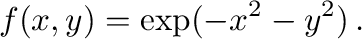
Figure 2:
A graph of a function in two variables. Note that we use a
gray-scale colors to for reproduction on standard laser printers; for
screen output there are visually more appealing color maps.
|
9.2 Function plotting in 3D
The following is an example for plotting the graph of the function of
two variables
The output is shown in Figure 2
  #! /usr/bin/env python3

  from pylab import *
  from mpl_toolkits.mplot3d import Axes3D

  figure()
  ax = subplot(111, projection='3d')

  x = linspace(-3,3,40)
  xx, yy = meshgrid(x,x)
  zz = exp(-xx**2-yy**2)

  ax.plot_surface(xx, yy, zz,
                  rstride=1,
                  cstride=1,
                  cmap=cm.binary,
                  edgecolor='k',
                  linewidth=0.2)

  ax.set_xlabel(r'$x$')
  ax.set_ylabel('$y$')
  ax.set_zlabel('$z$')
  title(r'The function $z=\exp(-x^2-y^2)$')
  savefig('plot3d.pdf')
  show()
Stability of a numerical method for solving ordinary differential
equations is of great theoretical and practical importance. A
necessary condition that any method has to satisfy is
zero-stability--it asserts that small perturbations in the initial
data will lead to bounded perturbations of the result in the limit of
small step size. Let us take the backward differentiation formula of
order (BDF6) as an example. To verify zero-stability, we have to
check that the roots of its first characteristic polynomial,
lie on or within the unit circle of the complex plane. For stiff
equations, the region of absolute stability is also important. It is
defined as the region of the complex  -plane in which the
stability polynomial, here
-plane in which the
stability polynomial, here
has roots of modulus no more than . For a thorough introduction to
these concepts, see [3]. So the computational tasks are:
- Plot the roots of the first characteristic polynomial with the
complex unit circle for comparison.
- Compute the root with the largest modulus and check if it
exceeds .
- Plot the region of absolute stability.
These tasks are accomplished by the following code; the resulting root
plot is shown in Figure 3 and the region of
absolute stability in Figure 4.
Figure 3:
Roots of  with the complex unit circle for comparison.
|
Figure 4:
The shaded area is the unbounded region in the complex -plane where BDF6 is absolutely stable.
|
  #! /usr/bin/env python3

  from pylab import *

  bdf6 = array([147, -360, 450, -400, 225, -72, 10])
  R = roots(bdf6)

  c = exp(1j*linspace(0,2*pi,200))

  figure()
  plot(R.real, R.imag, 'ko',
       c.real, c.imag, 'k-')
  title('Roots of the first characteristic polynomial for BDF6')
  savefig('zero-stability.pdf', bbox='tight')

  # It is known that 1 is a root, so we devide it out because the
  # root condition cannot be decided numerically in this marginal case.

  z1 = array([1,-1])
  reduced_bdf6 = polydiv(bdf6, z1)[0]

  if max(roots(reduced_bdf6))>1.0:
      print "BDF6 is not zero-stable"
  else:
      print "BDF6 is zero-stable"

  # Now lets plot the region of absolute stability

  rhs = array([60, 0, 0, 0, 0, 0, 0])

  def stabroots(z):
      R = roots(bdf6 - z*rhs)
      return max(abs(R))
  stabroots = vectorize(stabroots)

  x,y = meshgrid(linspace(-10,30,350),
                 linspace(-22,22,350))
  z = stabroots(x + 1j*y)

  figure()
  contour(x, y, z, [1.0], colors='k')
  contourf(x, y, z, [-1.0,1.0], colors=['0.85'])
  title('Absolute stability region for BDF6')
  grid(True)
  savefig('abs-stability.pdf', bbox='tight')

  show()
The Hilbert matrix is a standard test case for linear system solvers
as it is ill-conditioned, but has a known inverse [8]. We
shall test the default solver of Pylab as follows.
For each
 Hilbert matrix
  where
where
 compute
the solution to the linear system
compute
the solution to the linear system  ,
,
 .
Calculate the error and the condition number of the matrix and plot
both in semi-logarithmic coordinates.
.
Calculate the error and the condition number of the matrix and plot
both in semi-logarithmic coordinates.
  #! /usr/bin/env python3

  from pylab import *
  from scipy.linalg import hilbert, invhilbert

  def test (n):
      H = hilbert(n)
      b = ones(n)
      return norm(solve(H,b) - dot(invhilbert(n),b)), cond(H)

  test = vectorize(test)

  nn = arange(1,16)
  errors, conds = test(nn)

  figure()
  semilogy(nn, errors, '-',
           nn, conds, '*')
  legend(('Error',
          'Condition Number'),
         loc = 'lower right')
  title('Hilbert matrix test case for numpy.linalg.linalg.solve')
  show()
Calculate the least square fit of a straight line to the points
 , given as two arrays x and y. Plot the
points and the line.
, given as two arrays x and y. Plot the
points and the line.
  #! /usr/bin/env python3

  from pylab import *
  from scipy.linalg import lstsq

  def fitline (xx, yy):
      A = c_[xx, ones(xx.shape)]
      m, b = lstsq(A, yy)[0]
      return m, b

  xx = arange(21)
  yy = xx + normal(size=xx.shape)
  m, b = fitline(xx, yy)

  figure()
  plot(xx, yy, '*',
       xx, m*xx+b, '-')
  legend(('Data', 'Linear least square fit'),
         loc = 'upper left')
  show()
A quantile-quantile plot (“Q-Q plot”) is often used in statistical
data analysis to visualize whether a set of measured or otherwise
generated data is distributed according to another, usually assumed,
probability distribution [9].
As an example, we compare samples a Poisson distribution (as synthetic
“data”) to the normal distribution with the same mean and standard
deviation (as the “model”); the result is shown in
Figure 5.
Figure 5:
Q-Q plot comparing the Poisson and the normal distribution.
|
  #! /usr/bin/env python

  from pylab import *

  p = poisson(lam=10, size=4000)
  m = mean(p)
  s = std(p)
  n = normal(loc=m, scale=s, size=p.shape)

  a = m-4*s
  b = m+4*s

  figure()
  plot(sort(n), sort(p), 'o', color='0.85',
       markeredgewidth=0.2, markeredgecolor='k',)
  plot([a,b], [a,b], 'k-')
  xlim(a,b)
  ylim(a,b)
  xlabel('Normal Distribution')
  ylabel('Poisson Distribution with $\lambda=10$')
  grid(True)
  savefig('qq.pdf', bbox='tight')
  show()
In one compares an empirical distribution against an assumed model
distribution, one does not need to resort to sampling the model, but
can use the percentage point function (PPF), which is the
inverse of the cumulative distribution function (CDF), when
available. In the above example, that would amount to replacing the
assignment of n by the following code:
  from scipy.stats import norm
  n = norm.ppf((0.5+arange(len(p)))/len(p), loc=m, scale=s)
(Since the resulting vector is already sorted, it also does not need
explicit sorting.) When available, the PPF is the preferred way of
doing the plot as avoids sampling uncertainty for the assumed model
distribution.
This document is loosely based on an introduction to Octave,
initially written by Hubert Selhofer [2]. Some additions were
provided by Miriam Grace.
- 1
-
E.W. Dijkstra,
Why numbering should start at zero, EWD 831,
E.W. Dijkstra Archive, University of Texas at Austin, 1982.
http://www.cs.utexas.edu/users/EWD/ewd08xx/EWD831.PDF
- 2
-
H. Selhofer, with revisions by M. Oliver and T.L. Scofield,
Introduction to GNU Octave.
http://math.jacobs-university.de/oliver/teaching/iub/resources/octave/octave-intro.pdf
- 3
-
E. Süli and D. Mayers,
“An Introduction to Numerical Analysis,”
Cambridge University Press, 2003.
- 4
-
Anaconda, accessed February 4, 2020.
https://www.anaconda.com/distribution/
- 5
-
Broadcasting, accessed September 9, 2012.
http://docs.scipy.org/doc/numpy/user/basics.broadcasting.html
- 6
-
NumPy for Matlab users, accessed February 4, 2020.
https://docs.scipy.org/doc/numpy/user/numpy-for-matlab-users.html
- 7
-
The Scipy Stack: Scientific Computing Tools for Python,
accessed June 6, 2013.
http://www.scipy.org/about.html
- 8
-
“Hilbert matrix,” Wikipedia, The Free Encyclopedia, 25 March 2012,
21:02 UTC.
http://en.wikipedia.org/w/index.php?title=Hilbert_matrix&oldid=483904783
- 9
-
“Q-Q plot,” Wikipedia, The Free Encyclopedia, 10 August 2012,
23:56 UTC.
http://en.wikipedia.org/w/index.php?title=Q
 . To increase this limit, use, e.g.,
![$[a,b]$](img5.png)


![\includegraphics[width=0.8\textwidth]{code/sinecosine.pdf}](img47.png)
![\includegraphics[width=0.8\textwidth]{code/plot3d.pdf}](img48.png)

![\includegraphics[width=0.8\textwidth]{code/zero-stability.pdf}](img52.png)
![\includegraphics[width=0.8\textwidth]{code/abs-stability.pdf}](img53.png)
![\includegraphics[width=0.8\textwidth]{code/qq.pdf}](img60.png)